 Skip to main content
Reversible Jump Markov Chain Monte Carlo (RJMCMC) Method

Jeremy Law contributed to the writing of this blog post
Continuing our series of blogs on methods of GI reserving that have caught our interest, we turn our attention to the Reversible Jump Markov Chain Monte Carlo (RJMCMC) stochastic reserving method.
This method was the subject of a paper by Gremillet et al. submitted for the Brian Hey prize at the 2013 GIRO conference, following other recent work from Verrall and Würthrich.
In this article, we summarise the novel approach it uses to estimate the distribution of reserves from a claims triangle and offer some of our own impressions.
What the Method does
We start with a well-established stochastic model for the claims triangle. Incremental payments in each cell are assumed to follow an Over Dispersed Poisson (ODP) distribution, the mean of which depends on the origin year (row) and development year (column). The column element of the parameters used is analogous to the development factors in the traditional chain ladder model, and the row element allows for different claim volumes in different underwriting years. A dispersion parameter, constant for the whole triangle, is used to adjust the variance of the claim distributions.
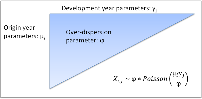
Note that strictly, this model doesn’t permit claims increments that are zero or negative, but there are ways of dealing with these cases. The model is extended by using an exponential function to give column parameters for the last few periods, as opposed to using a separate parameter for every development year.
The feature that sets Markov Chain Monte Carlo methods apart from other stochastic methods is that the parameters that define the distributions for incremental claims in the model are not estimated or sampled directly. Instead, the parameters themselves are randomly varied between simulations to reflect the parameter variance.
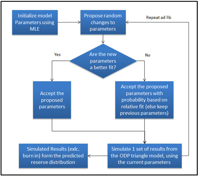
Having decided how the model is parameterised, and how parameters are to be updated, the following steps form the heart of the RJMCMC method:
- Initialise the model with arbitrary parameters, chosen, for example, using maximum likelihood estimation.
- Take the parameters used for the previous iteration of the method and update them using Gibbs sampling and the Metropolis-Hastings algorithm (discussed below).
- Simulate a set of results from the ODP triangle model based the selected parameterisation to allow for process error.
- Repeat steps 2) and 3) until a stable distribution emerges.
After a short ‘burn in’ period following initialising the model, parameters will equilibrate to wobbling around a roughly optimal set of parameters – their stationary distribution. Using each set of parameters it is possible to simulate a set of ultimate claims results with the ODP triangle model defined above. The range of results generated in this process, excluding results from the burn in period, is the distribution of results from the method.
This approach is rather convenient, as it means the same algorithm can be used to both refine the parameters in the model and to do the simulation itself to generate a distribution of results.
What does the name mean?
Next we give a brief explanation of some of the maths that underpins the above procedure and attempt to explain the slightly daunting name!
Markov Chain Monte Carlo (MCMC) methods are a way of randomly sampling from a probability distribution, based on constructing a Markov chain with a stationary distribution equal to this probability distribution.
The probability distribution that interests us in the case of this reserving problem is the joint distribution of the ODP triangle model parameters, conditional on the known data in the upper left half of the triangle. If we can sample sets of model parameter values from this then we have a good stochastic model of the claims triangle that neatly incorporates estimation variance. Unfortunately, this full joint distribution is too complicated to sample from directly, so normal Monte Carlo simulation techniques are not straightforward. However, by using Gibbs sampling and the Metropolis-Hastings algorithm to update parameters, it is possible to construct a Markov chain with the desired properties and use an MCMC approach.
Gibbs sampling is used to update the column and row parameters, and involves sampling from an assumed distribution based on parameters from the previous step of the algorithm. This works well if you can define a distribution for parameters, conditional on the other parameters in the model.
There is no simple assumed distribution for the parameters in the curve used for the tail, so instead the slightly more complex Metropolis-Hastings algorithm is used to update these. For this, you start with the parameters used for the previous iteration of the method and propose some random changes to them. You then evaluate the proposed new set of parameters using a “goodness of fit” function, which measures how well a given set of parameters describes the observed claims data, and this is compared against the previous parameters. The new parameters are kept if they are a better fit to the data than the previous set of parameters were. If they are a worse fit, then they are rejected with a probability that depends on their relative closeness; the worse the proposed parameters fit the data, the more likely they are to be rejected. Perhaps the most surprising feature of the algorithm is that the stationary distribution is the same, regardless of how changes to the parameters are proposed!
The method’s “reversible jump” prefix indicates an extension to the basic MCMC approach. In RJMCMC, changes in the dimensionality of the sample space (i.e. the number of parameters in the triangle model) from one simulation to the next are allowed for.
This is useful in the case of modelling the claims triangle as it opens up new possibilities for using a parametric function to approximate tail development factors. The more tail development periods the function is used to approximate development factors for, the fewer parameters are needed to model the remainder of the triangle. If the number of parameters to be sampled does not have to be constant from one sample to the next, then the number of periods of the triangle that are modelled by the tail function can be allowed to vary during the simulation. This allows the use of the tail to arrive at an “optimal” point without requiring a subjective decision from the user.
Impressions
The fundamental question is, “How useful are the results that the RJMCMC method gives you?” Ultimately, how well the method does will primarily depend on how good the data is, and how well the assumptions of the underlying ODP model hold up for the portfolio in question.
As with any more sophisticated method, there is the danger of losing sight of how the model comes up with its answers and falling into the “black box” mentality. It is important to understand what the method is doing and the relationships between the data, assumptions and results.
The GIRO paper goes on to compare results from the RJMCMC method with those from the traditional chain ladder Mack and Bootstrap methods. The means and coefficients of variations of reserves from the different methods are generally quite comparable, though the authors note that the use of a parametric tail distribution for the last few periods in their RJMCMC model can reduce the predicted variability of reserves compared to the other two methods.
It is worth noting that the RJMCMC approach is quite a general statistical tool that could be applied to a range of different models. For example, a lognormal rather than ODP model of incremental claims could be used, the parameter distributions could be assumed to take a different form, or, as explored in the GIRO paper, different types of tail distribution could be assumed. The RJMCMC approach is a useful method of taking these modelling assumptions and turning them into a distribution of results. It should prove to be a valuable piece of the reserving actuary’s toolkit going forward.